226 - Database Final
Lec8: View, Index, Procedure, Trigger
View
- Single table derived from other tables (base tables, views)
- DB object
- Under a schema (container): [schenaName.]viewName
- Virtual table: **★ Not necessarily has persistent data in physical form**
**★ View always up-to-date**
- Regular view: w/o persistent data
- Materialized view: w/ persistent data
View implementation
- Query modification approach ● Modify view query into a query on underlying base tables ● Cons: time-consuming to execute a view w/ complex queries
View materialization approach
● Create a temp table when first queried; better performance for subsequent Qs● INSERT, UPDATE, DELETE ➜ may modify persistent data of materialized view
● How to keep the table up to date?
 • whenever the base tables are modified

 • Incremental update
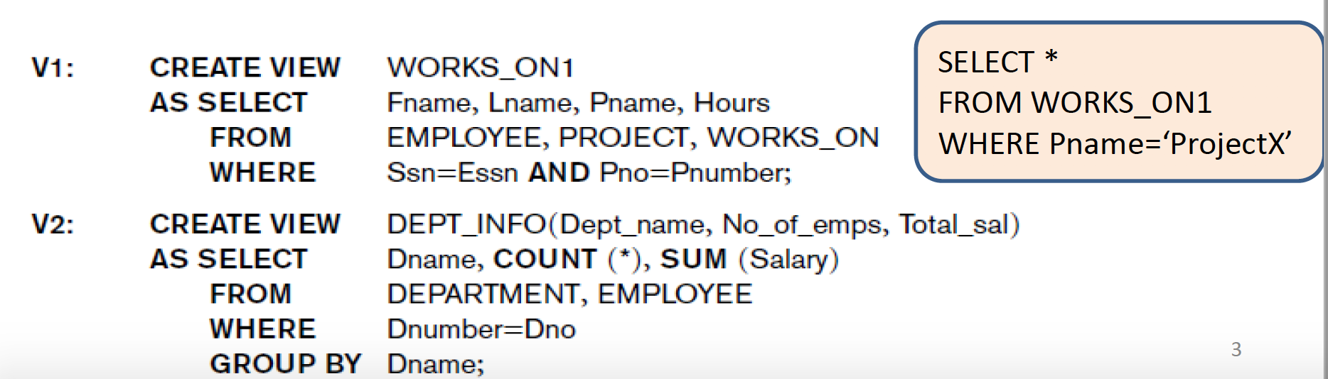
Insert/update/delete a view ➜ insert/update/delete a single base table w/o ambiguity
- No aggregation/grouping in view definition
- View columns include PK of base table
- View columns include all non
View w/ joining multiple tables: usually not possible
CREATE VIEW … WITH CHECK OPTION;
- Affected rows must satisfy WHERE clause in view definition
- Avoid this issue: inserting a row via view but the newly inserted row is not visible from the view
Index
CREATE INDEX empNameIdxON employee (name);
(( SELECT * FROM employee WHERE name = 'Bob'; ))
CREATE INDEX empNameDeptIdxON employee(name, dept);
(( SELECT * FROM employee WHERE name = 'Bob' AND dept='d2'; ))
- Separate persistent data structure for efficient accessing rows of table: DB object
- query optimization
- Under a schema (container): [SchemaName.]IndexName
- w/o appropriate index: table scan ➜ huge # of I/O ➜ slower
- w/ appropriate index: use index ➜ less # of I/O ➜ faster
- Different queries may benefit from different indexes
- Implementation: B+-tree, hash, etc
- ALTER, DROP
- Index is updated along with each INSERT/UPDATE/DELETE
- Adding index
- Proper index ➜ Optimize query
- Hurt insert/update/delete operations
- Consume space
Two single-column indexes vs one two-column index in MySQL?
If you have two single column indexes, only one of them will be used in your example.
If you have an index with two columns, the query might be faster (you should measure). A two column index can also be used as a single column index, but only for the column listed first.
Sometimes it can be useful to have an index on (A,B) and another index on (B). This makes queries using either or both of the columns fast, but of course uses also more disk space.
When choosing the indexes, you also need to consider the effect on inserting, deleting and updating. More indexes = slower updates.
- A single column in WHERE search condition
- Create an index if the ratio of data satisfying the condition is low
- If the ratio is high, a table scan (less # of I/O) may be better
- Multiple columns in WHERE search condition w/ AND
- Create a composite index for all columns in the search condition or more than one index (DB dependent)
- If the ratio is high, a table scan (less # of I/O) may be better
- Covering index: all columns in the query are included in index
- Performance implication: no need to fetch actual rows
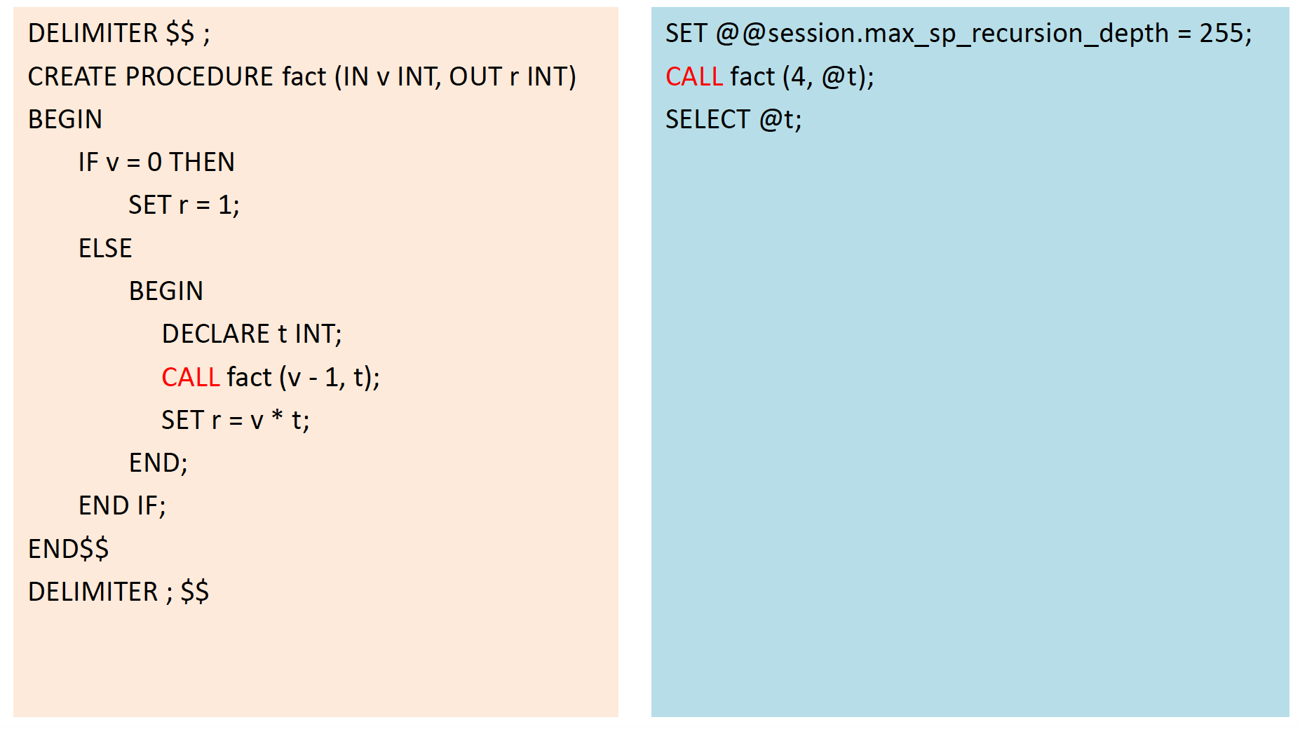
Stored Procedure
- Parameterized procedure in SQL: DB object
- Under a schema (container): [Schemaname.]ProcedureName
- Created once, executed repetitively
- In and/or out parameters, local variables
- Flow control: if, while, case, etc
Pros:
- Reduced server/client network traffic
- Stronger security: SP as gateway to control access
- Reuse/share of code (across different apps)
- Easier maintenance: grant permission on SP, not tables
- Improved performance (especially for MS SQL; but not so much in
Cons:
- Learning curve
- Difficult to migrate to different DBMS
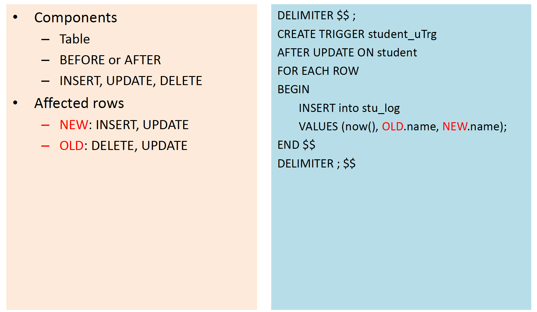
Triggers
Special SP automatically executed when DB INSERT/UPDATE/DELETE occurs
- Under a schema (container): [SchemaName.]TriggerName
- Event: table (view) & insert/update/delete, etc.
- Part of the transaction
Pros :
- Cascade changes through related tables
- guard against incorrect INSERT/UPDATE/DELETE, and enforce restrictions (beyond the CHECK)
- evaluate the state of a table before and after a modification and take actions based on that difference
- Central / global enforcement of business rules –rollback changes
Cons :
- Performance implication
- Learning curve
Lec9 : Functional Dependencies and Normalization
Guideline
Guideline 1: Entity & Attribute w/ Clear Semantic
- Each “obj” is represented as an entity
- Include only “related” attribute in an entity
- Easy to explain its meaning
- Do not combine multiple objects into a single relation
Guideline 2: No Anomalies
Anomalies example:
- Insert anomalies Need consistent info for department Cannot add a department w/o employees
- Deletion anomalies Delete the last employee for a department deletes department
- Update anomalies Change manager for department
Guideline 3: Avoid NULL Values
- Avoid frequent NULL
- NULL allowed under exceptional cases only
Guideline 4: No Spurious Tuples
Design schemas such that join attributes **are properly related (PK,FK)
Functional Dependencies (FD)
–Formal tool for analysis of relational schemas
–Detect / describe problems precisely
Definition X → Y
–X and Y: two sets of attributes of a relation R
- X: determinant Y: dependent
- ★ EachX value is associated with exactly one Y value
- ★ Different X values may be mapped to the same Y value
Given a populated relation R (a particular relation state r of R)
- Cannot determine which FDs hold and which do not (Unless meaning of and relationships among attributes known)
- Can state that FD does not hold if there are tuples that show violation of such an FD
➜ can determine may be true, and not true
A functional dependency FD: X → Y is called trivial if Y is a subset of X.
Normalization
Goals: Analyze relations based on FDs and PK to
- Improve schema design quality
- Reduce redundancy
- Minimize anomalies
Normal form: 1NF, 2NF, 3NF, BCNF, 4NF, 5NF
➜ The degree / level of how attributes are “related” in a relation
➜ A relation failed normal form tests is decomposed to smaller relations that satisfy the tests
Normalization through decomposition
Non additive join or lossless join: Extremely critical
\(It is the ability to ensure that any instance of the original relation can be identified from corresponding instances in the smaller relation\)Dependency preservation: Desirable may be sacrificed
Normal forms do not guarantee a good DB design
Necessary but avoid overdone
–Only up to 3NF, BCNF, or at most 4NF
– Too many small tables ➜ join operation implies poor performance
Superkey S : A subset of attributes S ⊆R, no two tuples t1 and t2 in any relation state r of R will have t1[S] = t2[S]
Key K : Minimal superkey: removal of any attribute from K will cause K not to be a superkey any more
R has > 1 keys, each key is a Candidate Key ==> prime attribute
–One is primary key
–Others are secondary keys
1st Normal Form (1NF): has PK and all non-PK attributes must depend on PK
– No multi-valued attribute and no nested relation
**– Flat relational model
**– Remove attrand place in separate relation (usually the best)
2nd Normal Form (2NF): 1NF + All non-key attributes must be fully FD on PK
–No partial dependencies. A partial dependency exists when a column is fully dependent on a part of a composite PK
– Left side of FD is part (proper subset) of PK of R
– Only applies to composite PK
– Move “problematic” attributes (and FDs) to a new relation
3rd Normal Form (3NF): 2NF + All non-key attributes must be directly FD on PK
–No transitive dependencies
Boyce-Codd Normal Form (BCNF): Every determinant in FD is a candidate key
– If there is only one candidate key, 3NF and BCNF are one and the same
– R is in BCNF if whenever a non-trivial FD X→A holds in R, then X is a super key of R
– May lose certain FDs
(For any A-> B, A should be a super key) (X A->B A is non-prime and B is prime)
•4th Normal Form (4NF): no multiple sets of multivalued dependencies
(1. A->>B for a single value of A, more than one of B exits
- Table should have at-least three columns
- For this table with A, B, C columns, B and C should be independent)
•5th Normal Form (5NF), or Project-Join Normal Form (PJNF): no pair wise cyclic dependencies
– deals w/ composite primary (candidate) key w/ ≥ 3 columns and join dependencies
•Domain Key Normal Form (DKNF) : No insertion, change, or data removal anomalies
Lec10 : Transaction
- A logical unit of DB processing that includes one or more operations (read –select, write –insert/update/delete)
- either completed in entirety or not done at all
- Boundaries
- begin transaction
- end transaction (commit or rollback)
ACID
- Atomicity
- A txn is an atomic unit of processing; either performed in its entirety or not performed at all
- Consistency
- Each txn takes the DB from one consistent state to another
- Isolation
- Each txn is executed in isolation from other txns
- Updates from a txn is not visible to others until it is committed
- Levels of isolation
- Durability
- Changes from a txn are permanent and never lost
- Cannot rollback a committed txn
COMMIT signals the successful end of a txn
– Any changes made by the txn should be saved
– These changes are now visible to other txns
ROLLBACK signals the unsuccessful end of a txn
–Any changes made by the txnshould be undone
–as if the txnn ever existed
The transaction manager enforces ACID
– commit and rollback used to ensure atomicity
– locks or timestamp are used to ensure consistency and isolation
– A log is kept to ensure durability
System log
Log == transaction log == journal
–Sequential, append-only persistent disk file
–Record operations of txn
–Write-ahead Logging (WAL)
Write into log first, and then write to DB
Log entries must be made before COMMIT processing can complete
Write (e.g., INSERT, UPDATE, DELETE)
–WAL: make a new log record before updating data pages
–Data pages may still in memory buffer (performance reason)
Commit
–WAL: make a new log record
–Flush all log records of the txn to disk
Checkpoint
–DB engine performs checkpoint periodically
–Flush all “dirty” data pages (committed or not) from buffer to disk
• Flush its corresponding log entry first
–A log record is made (on disk) of the txns that are currently running
–Why? Limit the amount of work during recovery
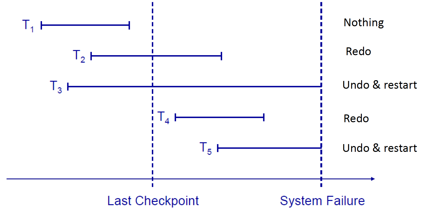
Undo: Replay log backward, replace DB data with old-value
Redo: Replay log forward, replace DB data with new-value
Backup: save {data and/or txn **log} to secondary storage
–Frequency
–Full: complete DB (data + txnlog) -time consuming
–Differential: delta since last full backup –size keeps increasing
–Incremental: delta since last any backup
•Chain: F1➜ i11➜ i12 ➜ i13 ➜ F2 ➜ i21 ➜ i22 ➜ i23 ➜ F3 ➜ …
•Chain: F1➜ i01 ➜ i02 ➜ d01 ➜ i11 ➜ i12 ➜ d02 ➜ i21 ➜ i22 ➜ F2 ➜ …
File system snapshot: not good enough for recovery ( May get un-update data)
Concurrency
If concurrency not allowed ➜ **run txns sequentially
Run txns concurrently ➜ interleave** their operations
Lost Update: Two txns accessing the same DB items have their operations interleaved in a way that makes value of DB item incorrect.
ex: Item X has an incorrect value because its update by T1 is lost (overwritten by T2)
Dirty Read: One txn updates a DB item, then read by 2nd txn, and then the 1st txn aborts
ex: Transaction T1 fails and must change the value of X back to old value, meanwhile T2 had read the temporary incorrect value of X.
Incorrect Summery: A txn calculates an aggregate summary function while other txns are updating the value
Unrepeatable reads: a row is read twice and the values differ between reads
Phantoms: Special case for Unrepeatable reads -- two identical reads return different set of rows
Ex. T1 reads a range of tableA ➜ T2inserts rows to the same range of tableA ➜ T1reads the same range of tableA
Schedule
– Operations in each Ti in S are in the same order in which they occur in Ti
–Operations from other txns Tj can be interleaved with the operations of Ti in S
| Notation | Meaning |
|---|---|
| b | begin_transaction |
| r | read_item |
| w | write_item |
| e | end_transaction |
| c | commit |
| a | abort |
★ Operations in a schedule are conflict if
- Belong to different txns, and
- Access the same item X, and
- At least one of those is write_item(X)
- operations could be all write_item(X)
– Conflict: r1(X) and w2(X), r2(X) and w1(X), w1(X) and w2(X)
– Not conflict:r1(X) and r2(X), w2(X) and w1(Y), r1(X) and w1(X)
Serial schedule:
– A schedule S is serial if, for every txn T in S, all the operations of T are executed consecutively in the schedule (w/o interleaving)
• Otherwise, the schedule is called nonserial schedule
– Every serial schedule is considered to be correct
• The order among txn in the schedule does not matter
– Some(not all) nonserial schedule gives correct result

Serializable Schedule:
A schedule S is serializable if it is equivalent to some serial schedule of the same n txns –A serializable schedule is correct
Schedule Equivalence :
- Result equivalent: too weak
- Conflict equivalence
- View equivalence
Conflict equivalence
–Two schedules are conflict equivalent if the order of any two conflicting operations is the same in both schedules
• Ex. The order “r1(X); w2(X)” is the same in both schedules
• If two conflicting operations are applied in different orders, the result can be different
Conflict serializable
–A schedule S is said to be conflict serializable if it is (conflict) equivalent to some serial schedule S’
•Non-conflicting operations in S can be reordered until S becoming the equivalent serial schedule
Testing Conflict Serializability
•Construct a precedence graph (serialization graph) and look for cycles
- Create a node in precedence graph for each txn
- Create an edge (Ti→ Tj) for each DB item
- Executing read_item(X) in Tjafter executing write_item(X) in Ti
- Executing write_item(X) in Tjafter executing read_item(X) in Ti
- Executing write_item(X) in Tjafter executing write_item(X) in Ti
The schedule S is serializable if and only if the precedence graph has no cycles


Serial schedule is serializable
–No interleaving, inefficient processing, low cpu%
–Correct
Serializable schedule: not the same as being serial
–Interleaving, concurrency, efficient processing
–Also correct
Lec11 : Concurrency Control
- what In concurrent execution env, if T1conflicts with T2over a data item A, then CC decides if T1or T2should get the A and if the other txnis rolled-back or waits
- why
- Enforce serializability of schedules
- Enforce ACID: noninterference, isolation, consistency
- Resolve read-write and write-write conflicts
- How
- locking
- timestamps ordering
Locking
ensure serializability of concurrent txns
Before read/write any ‘resource’ (table, row, etc)
- a txn must first acquire a lock on that resource
- DBMS issues the lock request automatically (on behalf of txn)
- DBMS releases the lock afterwards automatically
Binary locks
–Atomic operations
- lock_item(X)
- unlock_item(X)
Shared/Exclusive locks (read/write locks)
–Atomic operations
- read_lock(X)
- write_lock(X)
- unlock(X)
–Read-lock: several txns can simultaneously read an item but no txn can modify the item at the same time
–Write-lock: one txn exclusive access to write to a resource
Binary locks and read/write locks
•Does not guarantee serializability of schedule
•Need additional protocol for serializability→ 2PL
Two-Phase locking
Two Phases: (all lockings precede the 1st unlock)
–Locking(growing or expanding or first) phase
- New locks can be acquired(including lock upgrade)
- None can be released
–Unlocking(shrinking or second) phase
- Existing locks can be released(including lock downgrade)
- No new lock can be acquired
Theorem: if every txni n a schedule follows 2PL, the schedule is guaranteed to be serializable
2PL Pros: guarantee serializability
2PL Cons
- limits concurrency ===> because a Transaction may not be able to release an item after it has used it.
- does not permit all possible serializable schedules
- Some serializable schedules are prohibited by 2PL
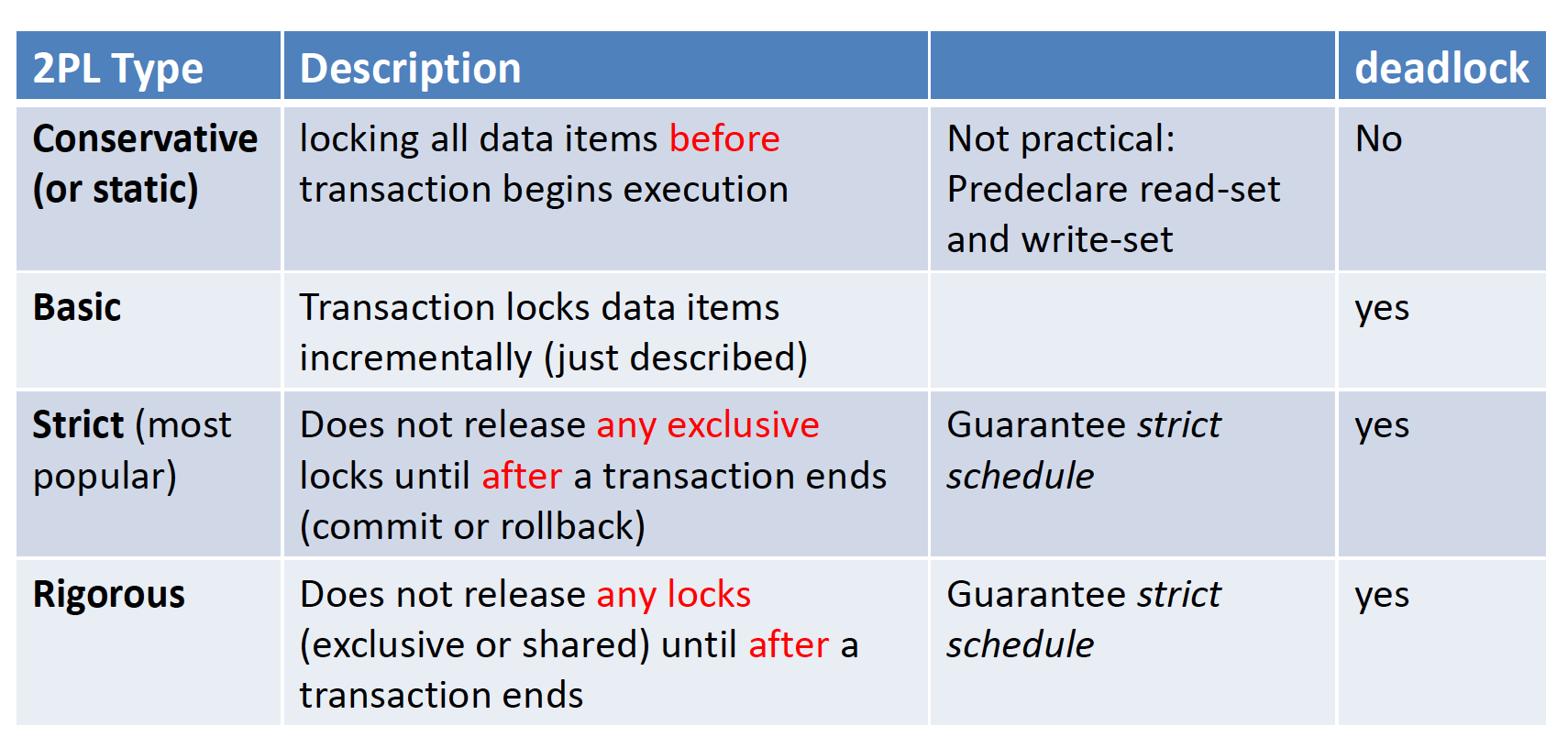
- deadlock is possible (except conservative 2PL)
- Basic 2PL - cascading aborts (why?)
- Fixed by strict 2PL & rigorous 2PL
Deadlock
Definition: each txn in a set of 2 or more txns waits for some item locked by some other txn
Deadlock detection and timeouts: more practical >>> Deadlock prevention
Deadlock Prevention
- Conservative 2PL
- locks all data items in advance before execution begins
- No deadlock since txn never waits for a data item
- Total Ordering all DB items; lock each in that specific order
- No deadlock. Not practical
- Transaction timestampTS(T) based
- Wait-die: older txn is allowed to wait for younger one; younger txn requesting an item held by older one is aborted and restarted with the same timestamp
- Wound-wait: younger txn is allowed to wait for older one; older txn requesting an item held by younger one aborts younger one and restarts it with the same timestamp
- Always aborts the younger one which may be involved in deadlock
- (+): No deadlock, no starvation
- (-): needless aborts/restarts
Deadlock Detection
- Deadlocks are allowed to happen
- Good for short txns and only locks a few items
- Wait-for graph
Starvation
Starvation: when a particular txn consistently waits or restarted and never gets a chance to proceed further
wait-die and wound-wait: no starvation ➜ Txn is restarted with the same timestamp
Timestamp Ordering (TO)
- Timestamp: A monotonically increasing integer
- The age of an operation or a transaction
- Larger TS: a more recent (younger) event or operation
- Timestamp ordering (TO)
- Timestamp (TS) monotonically increases
- TS assigned to a txn T when T starts, i.e., txn starting time TS(T)
- Order txns based on their TS
- Schedule w/ TO is serializable
- The only equivalent serial schedule: the order of txn timestamp values
Basic Timestamp Ordering
When two conflicting op occurring in incorrect order, reject the later **of the two by aborting the older ➜ younger txn takes precedence
Basic TO Algorithm
–T issues write_item(X)
- If read_TS(X) > TS(T) or if write_TS(X) > TS(T), then an younger txnhas already read the data item so abort and roll-back T and reject the operation. Restart T with a newTS.
- else execute write_item(X) of T and set write_TS(X) to TS(T)
–T issues read_item(X) :
- If write_TS(X) > TS(T), then an younger txn has already written to the data item so abort and roll-back T and reject the operation. Restart T with a new TS.
- If write_TS(X) ≤ TS(T), then execute read_item(X) of T and set read_TS(X) to max(TS(T), current read_TS(X))
– (+): No deadlock, conflict serializable
– (-) : cascading rollback, cyclic restart, starvation
• Neither 2PL nor basic TO allows all possible serializable schedules
Multiversion Concurrency control
Concept:
- maintains a number of versions of a data item
- read: from the appropriate version –never blocked
- write: to a new version
- Pros: serializability
- Cons: significantly more storage (recovery may need older versions)
Multiversion schemes
- Based on timestamp ordering: Google Spanner
- Based on 2PL
read_TS(Xi): read TS of Xi-the largest of all TSs of txns that have successfully read version Xi
write_TS(Xi): write TS of Xi that wrote the value of version Xi
(+): read is always successful, serializable
(-): cascading rollback, unless T cannot commit until all